1 Overview and goals

tl;dr: I just want the code.

This document details how you can understand segment usage in Adobe Analytics Workspace projects, without the need of APIs. This is possible due to a change made by the Adobe folks earlier this year (with the launch of Multiple Report Suites) which resulted in component usage being surfaced in the browser console.

The goal of this work is to create an R environment, to which you can load Workspace data into, allowing you to determine where components (e.g. Segments) are used across all of your Adobe Analytics Workspace projects. N.B. I am by no means an expert in R. I know a little, which places me firmly in the dangerous category.

1.1 Example use cases

You are keen to find out if users are using that hot new segment you have built out.
You want to ensure that users are applying a must have segment onto all of their Workspace projects (if so, you should give some thought to using a Virtual Report Suite).
You have discovered a segment which is flawed and you need to urgently identify all the projects currently using it, so that you can reach out to the project owner.
You have identified duplicate segments and need to understand which segment to retain based on its usage so that you can initiate retirement of the other segment.

1.2 Pre-requisites

Basic knowledge of R syntax
RStudio. It’s a great IDE for R
An Adobe Analytics user account
Admin access to ‘Show all’ projects in Components>Projects (recommended)
A modern browser with access to Developer tools

1.3 Time outline

Allow up to 1 hour to work through this example. To refresh the datasets at any point it takes around 15 mins.

2 Getting started

Firstly, load the required libraries.

# Load required libraries
library(jsonlite) # flexible, robust, high performance tools for working with JSON in R
library(dplyr) # a fast, consistent tool for working with data frame like objects
library(purrr) # tools for working with functions and vectors
library(splitstackshape) #tools for reshaping data
library(kableExtra) # build common complex tables and manipulate table styles
library(listviewer) # allows you to expose list exploration in a rendered .Rmd document
library(ggplot2) # an implementation of the Grammar of Graphics
library(lubridate) # tools to work with dates and times

Set your environment time zone (this should be your local timezone. In this example I have set mine to GB-Eire).

# Set env time
Sys.setenv(TZ='GB-Eire')

Create some folders in your working directory to save down the JSON files and to export any datasets to.

# Create directory folders
dir.create("Inputs", showWarnings = FALSE) # to save JSON files into
dir.create("Outputs", showWarnings = FALSE) # to save any export files into

2.1 Datasets

Component usage datasets are not (at the time of this article) available via the API. However, we can obtain the data we need via the JSON files which are surfaced to build the View project interface within Adobe Analytics.

JavaScript Object Notation (JSON) is the most common data format used for asynchronous browser/server communication. Most web APIs limit the amount of data that can be retrieved per request. If the client needs more data than what can fits in a single request, it needs to break dow the data into multiple requests that each retrieve a fragment (page) of data, not unlike pages in a book. As such, you may have more than one JSON file being surfaced, largely dependant on the number if Workspace projects you have!

2.2 Download JSON files

This step is the most manual part of the entire process and is largely dependant on how many Workspace projects you have. However, it takes <1 minute per JSON file so in the grand scheme of things (& the advantages of not having to wrestle with APIs) it is still relatively fast.

Launch Chrome and open Developer tools (View>Developer>Developer tools)
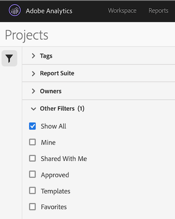
Log into Adobe Analytics and browse to Components>Projects. If you want to examine ALL projects then ensure you click the ‘Show All’ filter (admin rights required)

Within the Network tab of developer tools, filter for *‘?locale=en_US&expansion=‘* and file type ’xhr’. This should return something akin to this:

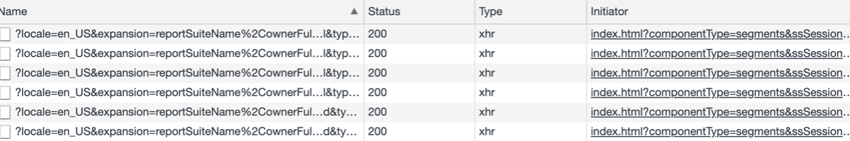
Remember - the number of results is dependant on the number of projects you have as each result has a 1k limit i.e. Each individual json response will contain data for up to 1,000 workspace projects. So if you have 4,200 workspace projects you can expect to see up to 5 json responses.

Click into the first entry and open the Response tab: You can see that JSON is used to represent the data in the UI.

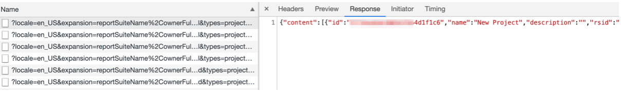
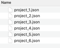
Copy the contents of the Response tab for each entry and save as a .json file into your ‘Inputs’ folder which we created earlier. For the purpose of this example I have saved the json files as project_1.json, project_2.json etc.

Knitr, by default, looks in the same directory as your .Rmd file to find any files you need to draw in, like data sets or script files. If you keep your data files and scripts in separate folders (and you should) you need to switch to that folder. Here we create some directory paths to make it easier to switch between:

# Create directory paths for ease of use
filedir <- getwd()
filedir_inputs <- file.path(filedir,"Inputs")
filedir_outputs <- file.path(filedir,"Outputs")

Then we check we can see the JSON files by returning a listing of the saved files within the Inputs folder. If you dont see the files, check you have saved the JSON files into the Inputs folder.

# Return the files within the Inputs folder
dir(filedir_inputs)

## [1] "project_1.json" "project_2.json" "project_3.json" "project_4.json"
## [5] "project_5.json" "project_6.json"

Next, we want to create a character vector of all the json files above using list.files().

# Create a character vector of the names of the json files above using list.files().
json_filenames <- list.files(filedir_inputs, pattern="*.json", full.names=TRUE)
json_filenames

3 Understanding the data

To read JSON data, we are using the fromJSON function from the jsonlite package. For the purpose of this tutorial I have used sample data.

Let’s read in one of the data files and understand the content.

# Pull in the first json file to inspect it
json_file1 <- fromJSON(json_filenames[1], simplifyVector = FALSE)

# Look at the first json file
glimpse(json_file1, max.level = 1)

## List of 11
##  $ content         :List of 1000
##  $ number          : int 0
##  $ size            : int 1000
##  $ numberOfElements: int 1000
##  $ totalElements   : int 3272
##  $ previousPage    : logi FALSE
##  $ firstPage       : logi TRUE
##  $ nextPage        : logi FALSE
##  $ lastPage        : logi FALSE
##  $ sort            : NULL
##  $ totalPages      : int 4

We observe the file is a list with 11 components. The other important point is that ‘$content’ is another list. This content component sounds promising…Let’s inspect.

# Look at the first json file $content
glimpse(json_file1$content[[1]])

## List of 16
##  $ id                : chr "5a1708f9bdf14b3152f7889a"
##  $ name              : chr "Performance - Daily Report"
##  $ description       : chr "Project Information"
##  $ rsid              : chr "myreportsuite"
##  $ reportSuiteName   : chr "My Report Suite"
##  $ owner             :List of 3
##   ..$ id   : int 200060001
##   ..$ name : chr "Kelly Preston"
##   ..$ login: chr "kpreston"
##  $ companyTemplate   : logi FALSE
##  $ type              : chr "project"
##  $ externalReferences:List of 4
##   ..$ dateRangeIds       :List of 2
##   .. ..$ : chr "yesterday"
##   .. ..$ : chr "4egad15155bf155cfbf23f76"
##   ..$ calculatedMetricIds:List of 2
##   .. ..$ : chr "cm1234_593179c897301a62eb9dd4e5"
##   .. ..$ : chr "cm1234_5a2ffab77245ec60b43d33bd"
##   ..$ rsids              :List of 1
##   .. ..$ : chr "vrs_prod1"
##   ..$ segmentIds         :List of 3
##   .. ..$ : chr "556c2cd5e4b0149fbcc252ba"
##   .. ..$ : chr "s1234_58948dfee4b04679ce03ed44"
##   .. ..$ : chr "54d9d5cce4b093ca5b708805"
##  $ tags              :List of 3
##   ..$ :List of 3
##   .. ..$ id        : int 19500
##   .. ..$ name      : chr "Product A"
##   .. ..$ components: list()
##   ..$ :List of 3
##   .. ..$ id        : int 21805
##   .. ..$ name      : chr "GI"
##   .. ..$ components: list()
##   ..$ :List of 3
##   .. ..$ id        : int 48762
##   .. ..$ name      : chr "BAU Reporting"
##   .. ..$ components: list()
##  $ shares            :List of 2
##   ..$ :List of 7
##   .. ..$ shareId           : int 3642472
##   .. ..$ shareToId         : int 200075739
##   .. ..$ shareToType       : chr "user"
##   .. ..$ componentType     : chr "project"
##   .. ..$ componentId       : chr "5a1708f9bdf14b3152b6787a"
##   .. ..$ shareToDisplayName: chr "John Musk"
##   .. ..$ shareToLogin      : chr "jmusk"
##   ..$ :List of 7
##   .. ..$ shareId           : int 5042587
##   .. ..$ shareToId         : int 200137280
##   .. ..$ shareToType       : chr "user"
##   .. ..$ componentType     : chr "project"
##   .. ..$ componentId       : chr "5a1708f9bdf14b3152b6787a"
##   .. ..$ shareToDisplayName: chr "Henry Peters"
##   .. ..$ shareToLogin      : chr "hpeters"
##  $ approved          : logi FALSE
##  $ favorite          : logi FALSE
##  $ siteTitle         : chr "My Report Suite"
##  $ modified          : chr "2020-04-27T14:47:01Z"
##  $ created           : chr "2017-11-23T17:44:25Z"

This looks like what we are after! It is a list with information on 1,000 projects. Each contains 16 named components of various lengths and types.

We can see there are further lists contained this list- ‘owner’ and ‘externalReferences’. Let’s take a closer look at each, starting with owner.

# Look at the first json file $content$owner
glimpse(json_file1$content[[1]]$owner, max.level = 1)

## List of 3
##  $ id   : int 200060001
##  $ name : chr "Kelly Preston"
##  $ login: chr "kpreston"

OK so it contains the user ID, name and login. Next, take a look at externalReferences:

# Look at the first json file $content$externalReferences
glimpse(json_file1$content[[1]]$externalReferences, max.level = 1)

## List of 4
##  $ dateRangeIds       :List of 2
##  $ calculatedMetricIds:List of 2
##  $ rsids              :List of 1
##  $ segmentIds         :List of 3

Another list. So, this is where our components are stored- Date Ranges, Calculated Metrics and Segments. A list within a list within a list…“Downward is the only way forward”.

Let’s have a look into what is contained with ‘segmentIDs’ (for the first project):

# Examine SegmentIDs for the first project
glimpse(json_file1$content[[1]]$externalReferences$segmentIds, max.level = 1)

## List of 3
##  $ : chr "556c2cd5e4b0149fbcc252ba"
##  $ : chr "s1234_58948dfee4b04679ce03ed44"
##  $ : chr "54d9d5cce4b093ca5b708805"

Those are segment IDs.

As we have seen above, $externalReferences contains important variables.

The listviewer package allows you to expose list exploration in a rendered .Rmd document. It is sometimes easier to understand the structure of a json file by looking at that. Let’s run it.

# Run listviewer on json_file1
listviewer::jsonedit(json_file1)

You can see that JSON stores data in Arrays (denoted by [square brackets]) or Objects (denoted by {curly brackets}). We now know we want to take in the $content component from each of the saved json files.

Having inspected and understood the data we can now import all the data. We can write a simple loop that automatically downloads and combines many files.

# Loop and import all json files
projects_raw <- list()
for(i in 1:length(json_filenames)){
  datatmp <- fromJSON(json_filenames[i], simplifyVector = FALSE)$content
  listtmp = datatmp
  projects_raw = c(projects_raw, listtmp)
}

# Remove environment objects which are no longer required.
rm('json_file1', 'listtmp', 'datatmp', 'i')

Let’s take a look at the number of elements in the list (i.e. the number of Workspace projects we have the data for).

# Understand size
length(projects_raw)

## [1] 4383

And, if you want, inspect the entire list using listviewer to ensure we have what we need and there are no issues within the files.

You will see that each of the entries has numeric indexing. I’d rather have each element in the list be named by the project it refers to. So let’s do that. Here we use purrr::map(), which is a function for applying a function to each element of a list - similair to lapply().

# Rename elements
projects_raw %>%
  rlang::set_names(map_chr(.,'name')) %>%
  listviewer::jsonedit()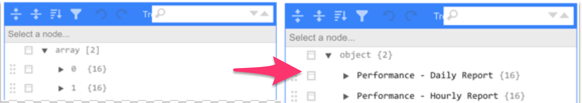

4 Extracting data

4.1 Project summary data

Create a new dataframe with the main project elements. It is safer, (albeit more cumbersome) to explicitly specify type and build your data frame the usual way.

We will take the Project ID, Project name, RSID, RS name and the dates the project was created and last modified.

# Create Projects df 
projects_df <- projects_raw %>% {
  tibble(
    project_id = map_chr(., "id"),
    project_name = map_chr(., "name"),
    rsid = map_chr(., "rsid"),
    report_suite_name = map_chr(., "reportSuiteName"),
    date_created = map_chr(., "created"),
    date_modified = map_chr(., "modified")
  )
}

Let’s inspect the dataframe contents.

# Number of rows
nrow(projects_df)

## [1] 4383

# Number of unique project Ids
length(unique(projects_df[["project_id"]]))

## [1] 3272

You may see a discrepancy between the number of rows and the number of unique Project Ids. As previously mentioned, if you copy in all the JSON responses you can often see the same page twice. Let’s remove the duplicates. The number of rows should now equal the number of Project IDs.

# Remove duplicates
projects_df <- unique(projects_df)

# Number of rows
nrow(projects_df)

## [1] 3272

Next I want to fix the dates. The dates are Pacific time. I want to change these to my local timezone of GMT.

# Created date
projects_df$date_created <- as.POSIXct(projects_df$date_created, "%Y-%m-%dT%H:%M", tz="America/Los_Angeles")  
attributes(projects_df$date_created)$tzone <- "GB-Eire"

# Modified date
projects_df$date_modified <- as.POSIXct(projects_df$date_modified, "%Y-%m-%dT%H:%M", tz="America/Los_Angeles")  
attributes(projects_df$date_modified)$tzone <- "GB-Eire"

You can see that both these date fields are Date/Time (dttm). So, I am going to create a new field just to contain the created on date, which makes it easier for any analysis & plotting.

# Rename existing columns
names(projects_df)[5] <- "date_created_dttm"
names(projects_df)[6] <- "date_modified_dttm"

# Create a new Created date (date only) field
projects_df$date_created <-as.Date(projects_df$date_created_dttm)

# Check the date field types
glimpse(projects_df)

## Rows: 2
## Columns: 7
## $ project_id         <chr> "5a1708f9bdf14b3152f7889a", "5a2e12e41eadd43d7862d…
## $ project_name       <chr> "Performance - Daily Report", "Performance - Hourl…
## $ rsid               <chr> "myreportsuite", "myreportsuite"
## $ report_suite_name  <chr> "My Report Suite", "My Report Suite"
## $ date_created_dttm  <dttm> 2017-11-24 01:44:00, 2017-12-11 22:15:00
## $ date_modified_dttm <dttm> 2020-04-27 22:47:00, 2020-03-25 17:55:00
## $ date_created       <date> 2017-11-24, 2017-12-11

4.2 Project segment usage

Extract the project id, project name, rsid and a list of the segment ids that each project is using.

# Create Segments df
segments_df <- tibble::tibble(
  project_id = map_chr(projects_raw, "id"),
  project_name = map_chr(projects_raw, "name"),
  rsid = map_chr(projects_raw, "rsid"),
  project_segments = projects_raw %>% 
    map("externalReferences") %>% 
    map("segmentIds") %>%
    map_chr(~ paste(.x, collapse = ","))
)

We now need to split the segments i.e. so that one row contains one project id and one segment id. We use the function cSplit from splitstackshape to accomplish this.

# Split segment column
segments_df <- cSplit(segments_df, 
                      "project_segments", sep = ",", direction = "long")

# Give the segment column a more appropriate name
names(segments_df)[4] <- "segment_id"

# Take a quick look at the Segment df
kable(head(segments_df)) %>%
  kable_styling(bootstrap_options = c("striped", "hover", "bordered")) %>% 
row_spec(0, bold = T, color = "white", background = "#2c3e50")

project_id	project_name	rsid	segment_id
5a1708f9bdf14b3152f7889a	Performance - Daily Report	myreportsuite	556c2cd5e4b0149fbcc252ba
5a1708f9bdf14b3152f7889a	Performance - Daily Report	myreportsuite	s1234_58948dfee4b04679ce03ed44
5a1708f9bdf14b3152f7889a	Performance - Daily Report	myreportsuite	54d9d5cce4b093ca5b708805
5a2e12e41eadd43d7862db6a	Performance - Hourly Report	myreportsuite	54d9d5cce4b093ca5b708805
5a2e12e41eadd43d7862db6a	Performance - Hourly Report	myreportsuite	s1234_5787aaabe4b0f9d1f7aa9519
5a2e12e41eadd43d7862db6a	Performance - Hourly Report	myreportsuite	556c2cd5e4b0149fbcc252ba

And there we have it! A listing of the segments used in every Workspace project.

You may wish to output the list to a csv file for sharing amongst your team (this will export it into the Outputs directory we created earlier):

# Export segments_df as .csv to Outputs folder
write.csv(segments_df, file.path(filedir_outputs, "segment_usage.csv"), row.names=FALSE)

The above outlines the process understanding what segments are used across your Workspace projects. You can easily adapt the code to perform the same for Calculated metrics or date ranges or shares or tags…

5 Analysis

This part is purely optional and contains examples of some high level analysis you can perform on the data.

5.1 Segment use

Count the number of segments used in each workspace project:

# Number of Segments per Project
segments_df %>%
  group_by(project_id, project_name) %>%
  dplyr::summarize(
    total_segments = n()) %>%
  arrange(-total_segments)

## `summarise()` has grouped output by 'project_id'. You can override using the `.groups` argument.

(For anyone interested the highest number of segments I found applied to a single project was 328.)

Let’s flip that and look at the number of projects each segment has been used in:

# Number of Projects per Segment
segments_df %>%
  group_by(segment_id) %>%
  dplyr::summarize(
    total_projects = n()) %>%
  arrange(-total_projects)

(Again, for those interested I have a segment which is used across 2,872 workspace projects).

Tip: You may opt to restrict your search to a particular Report suite, if so just filter on rsid accordingly.

6 Conclusion

This document provides a way to determine where segments are used across Workspace projects. Please be aware that segments are used in other areas, for example, Data Warehouse extracts, Calculated metrics. As such, be careful using the above in your decision making process to delete Segments!

I am hopeful that A4A (Analytics 4 Analytics) or API upgrades will remove the need for this approach longer term, but for now, happy hunting.

6.1 Further work

The above can be built upon further, by bringing in additional data sets. For example, you can bring in data pertaining to each Segment, such as Segment name, Creation date, Owner, Last modified date.

You can accomplish this by using either the:

API
rSiteCatalyst package by Randy Zwitch E.g. segments <- GetSegments(rs$rsid).

With the segment data you can then pull in the segment name, for example:

## `summarise()` has grouped output by 'segment_id'. You can override using the `.groups` argument.

7 Feedback & Corrections

If you have any feedback to this post/you spot a mistake/wish to suggest changes, please send me an email to wayne [@] analyse.ie

8 R-Script

If you just want the code used in this example here you go.

Segment use - Adobe Analytics

July 2020